Power Beamforming (PBF) is another frequency-based mapping method in NoiseImage. It combines several advanced algorithmic beamforming approaches in one operating principle. Using eigenvalue decomposition of the cross-spectral matrix (CSM), the acoustic map is divided into single (pseudo) sources and their point-spread functions (PSF). An exponentiation of the PSF while applying opposite manipulation to the sound source strengths results in the attenuation of the side lobes and sharpens the main lobes. This in turn results in an increase of dynamic and a sharpening of the source representation.
The algorithmic method the calculation is based on is determined by the exponent \(ν\) which is selected with a slider. The further the slider is moved to the left, the more the sources are sharpened and the dynamic are increased. To obtain meaningful results, however, a sufficiently large time range must be selected.
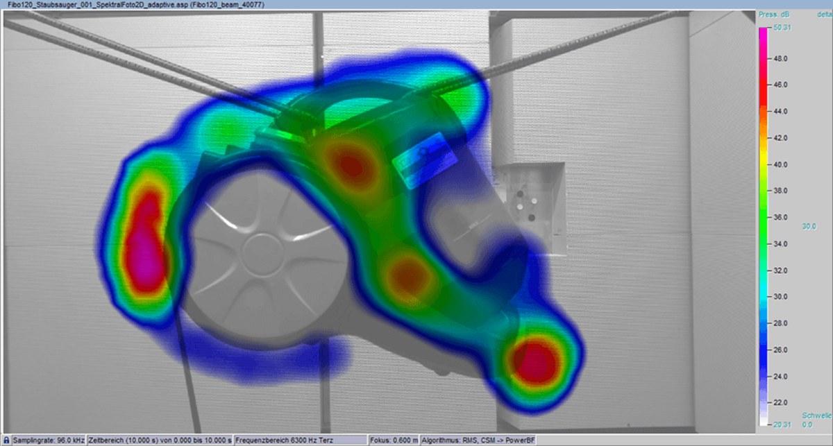
- Slider far left:
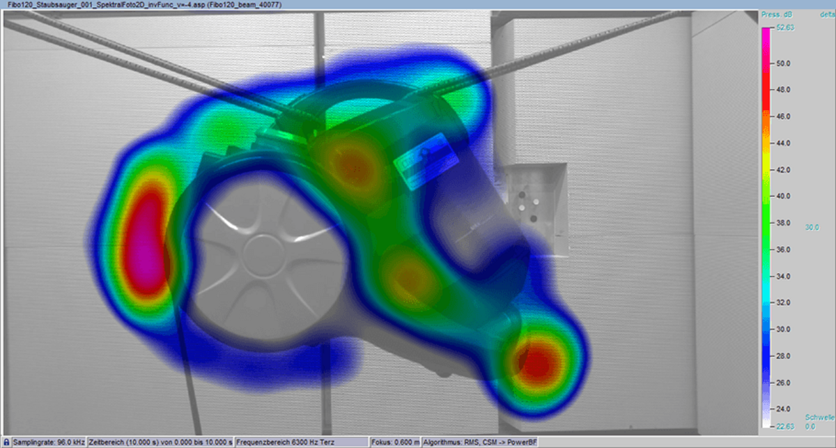
\(ν=-1\) corresponds to adaptive beamforming (Minimum Variance Beamforming1) - Slider in the left half:
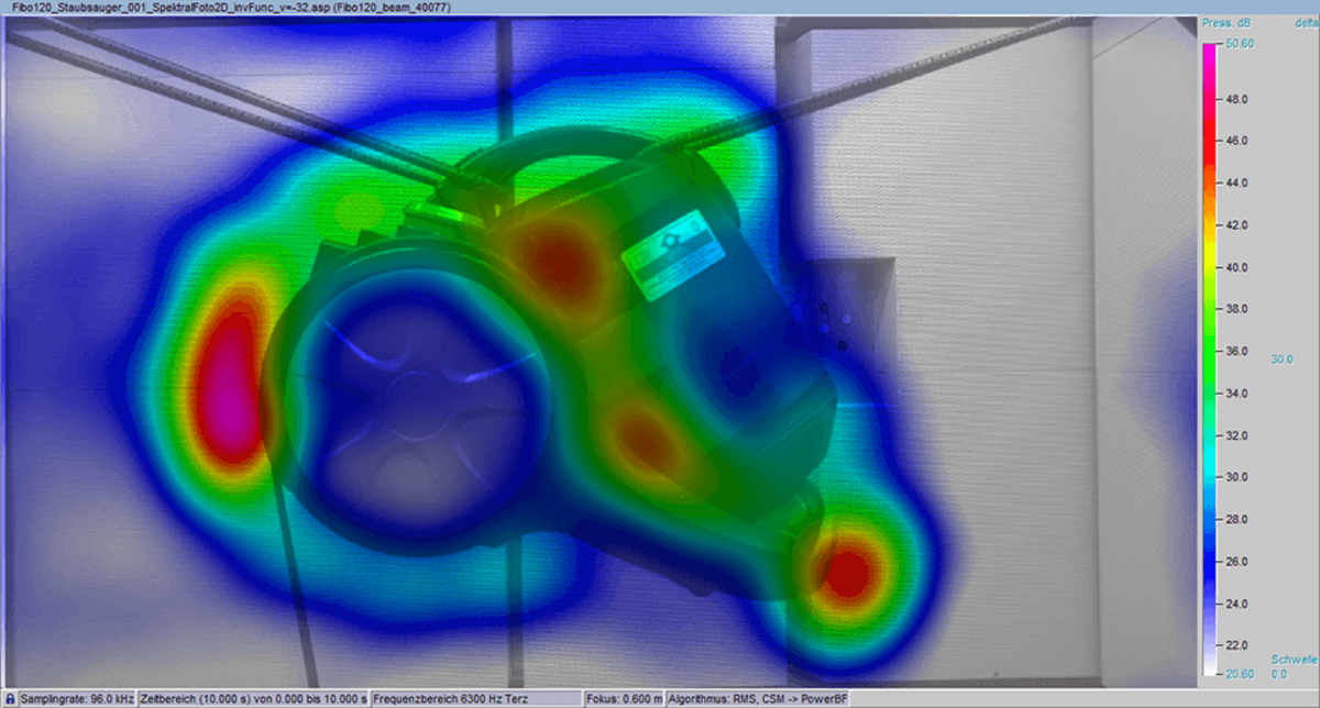
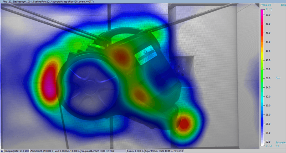
\(-1<1/ν<0\) with defined -2,-4,-8,-16 and -32 is here called inverse functional beamforming - Slider in middle position:
\(ν=∞\) is here called asymptotic beamforming - Slider in the right half:
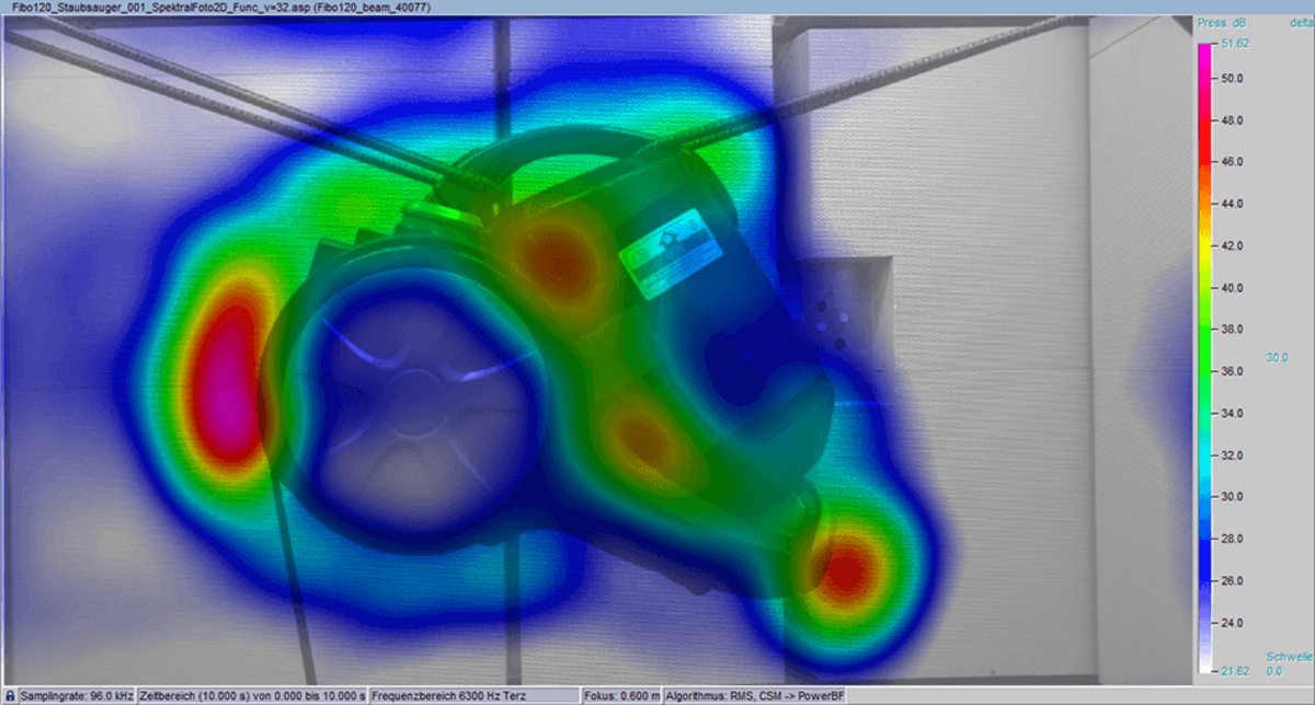
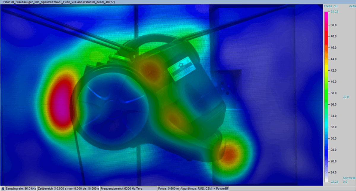
\(0<1/ν<1\) with defined 2,4,8,16 and 32 corresponds to functional beamforming - Slider far right:
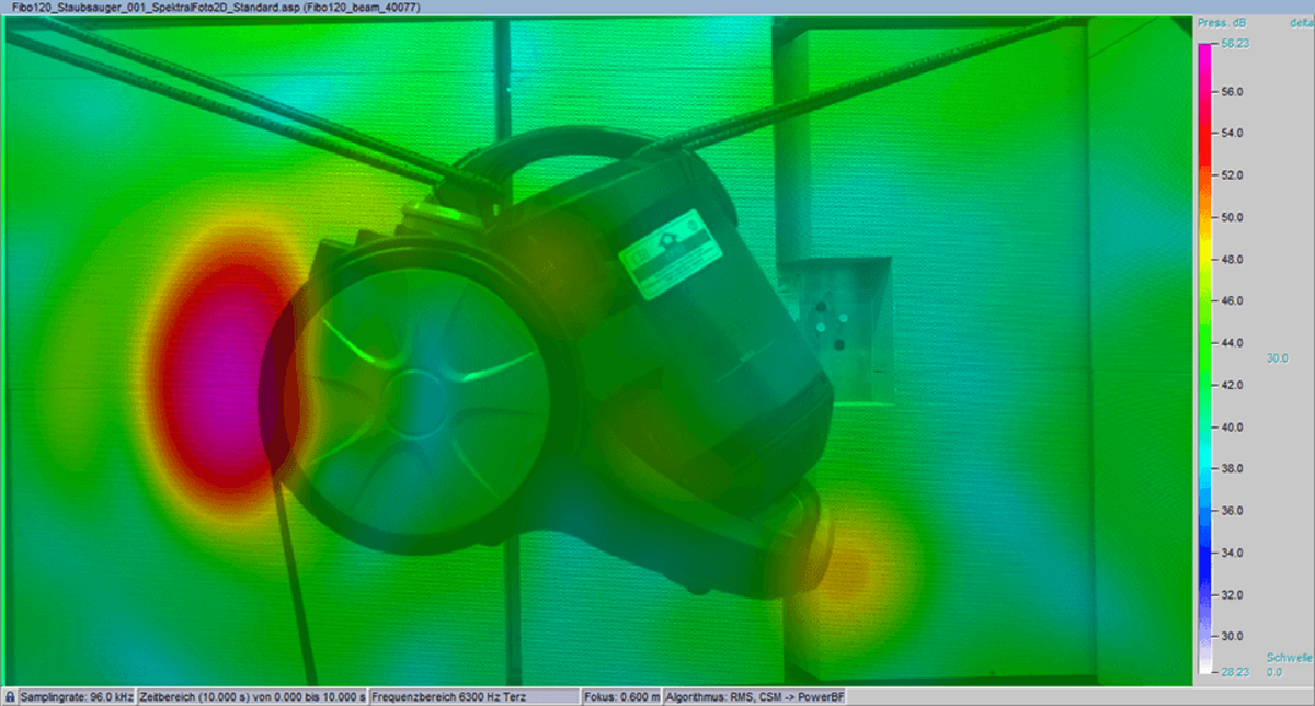
\(ν =1\) corresponds to standard beamforming based on the cross spectral matrix