Orthogonal Beamforming (OBF)

How does Orthogonal Beamforming work?

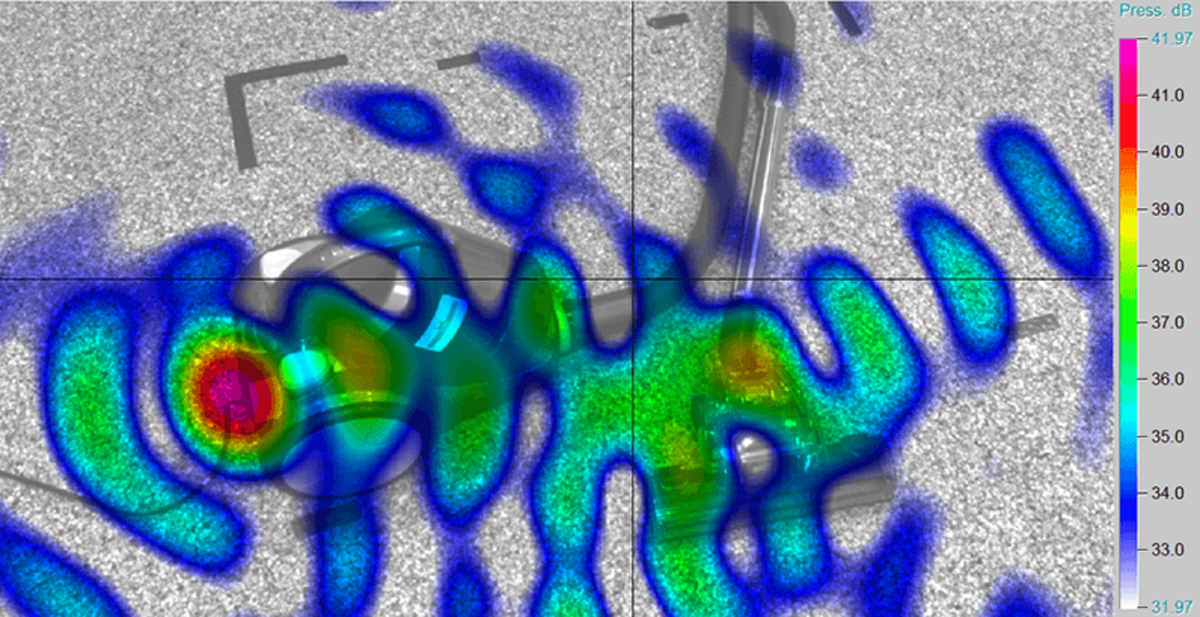
In a real measurement environment, a sound field usually consists of a superposition of many independent sound sources which are caused by simultaneously occurring mechanical, thermal and aerodynamic processes. Due to the characteristics of conventional beamforming, it might not be possible to map all sources separately.

A method that improves source representation algorithmically is OBF. It uses the effect that sources can be tracked back to orthogonal eigenvectors of the cross spectral matrix $C$which enables a separation of sources. The separation results from the decomposition of $C=V\Lambda V^H$in its diagonal matrix of eigenvalues $\Lambda$, its matrix of eigenvectors $V=[V_1,\dots,V_N]$ and its transposed-conjugate matrix $V^H$. Therefore, the $i$-th component of the cross spectral matrix $C_i$is calculated like:

$$C_i=\Lambda_{ii}V_i{V_i}^H,\qquad C=\sum_iC_i.$$

For the decomposition, it is assumed that the single non-coherent main sound sources are represented by the highest eigenvalues while all other eigenvalues are caused by random noise. The total number of components corresponds to the number of microphones $N$ of the array. With the $i$-th calculated cross spectral Matrix $C_i$it is possible to apply a conventional beamforming approach $B_i(\vec{x},\omega)$:

$$B_i(\vec{x},\omega)=g^H(\vec{x},\omega)C_ig(\vec{x},\omega).$$

Since sources can be mapped separately this way, OBF is preferably used for complex sound fields as found in machine noise. Furthermore, the approach leads to an identification of sound pressure levels of a source more accurate than attained with conventional beamforming methods and without increasing calculation time. In NoiseImage, it is possible to select a single component or a connected range of components. If all components are selected at once, the calculated map will be identical to the map calculated with conventional beamforming based on the cross spectral matrix $C$.

Example: Vacuum Cleaner

In the example, the first three components of OBF compared to normal FDBF are shown. A vacuum cleaner in a frequency range between 5.44 kHz and 6.14 kHz is used as sound source. The 1^st component shows a dominant source at the brush while the 2^nd component belongs to the noise emitted at the end of the tube. The source at the air outlet of the motor, which is shown in the 3^rd component, cannot be separated clearly from an artefact due to its low sound pressure level when using conventional FDBF.