The quality of beamforming depends on the size of the array and its microphone distribution. To specify a frequency range within which the array is suitable for locating sound sources, cut-off frequencies can be defined.
Lower Cut-off Frequency
The lower cut-off frequency depends mainly on the size of the array. Similar to optics, the term aperture is used in acoustics. In general, the larger the aperture of the array, the lower the frequencies that can be clearly localized. The 3 dB beamwidth width at an aperture angle of 180° can be used to define a lower cut-off frequency. This means at which frequency the 3 dB range of the beamwidth still fits into an acoustic map with infinite extension. This can be determined by calculating the cut-off frequency of the 3 dB beamwidth for different realistic beam angles and then interpolating it. Fig. 1 shows an example of the relationship between beamwidth and opening angle for the microphone array Ring48. Accordingly, the lower cut-off frequency for this array is 164 Hz. In practical applications, it is recommended to assume approximately twice this theoretic border.
Upper Cut-off Frequency
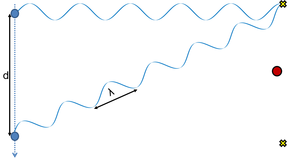
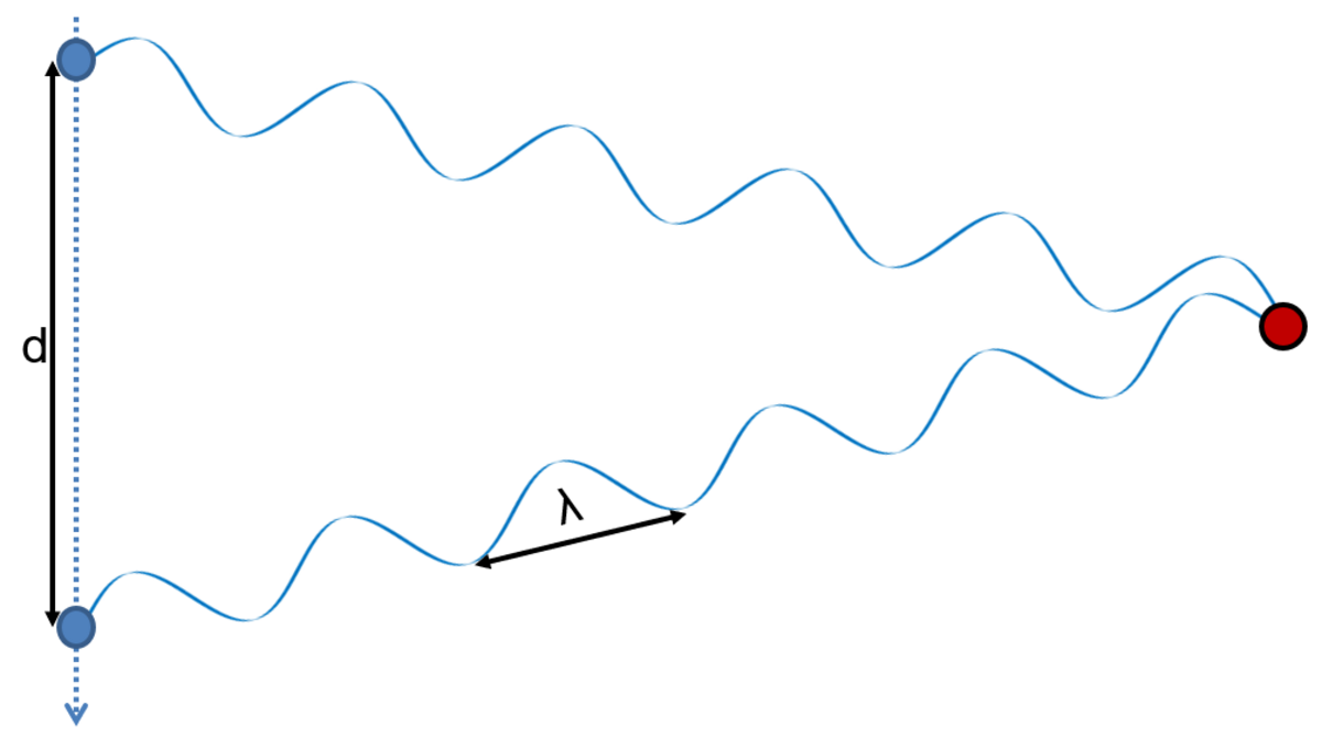
The upper frequency limit depends on the sampling rate \(fs\) and the distance between the microphones. According to the Nyquist-Shannon sampling theorem, the sampling rate of the data recorder must be at least twice as high as the highest frequency of the origin sound emission. If this is not adhered to, time aliasing occurs. This becomes noticeable by so-called alias signals which are generated due to under-sampling \(f > fs/2\). Alias signals are apparent signals with frequency components of\(f < fs/2\). The distance between the microphones determines the cut-off frequency at which spatial aliasing occurs. Fig. 2 illustrates this using the example of the localization of a source emitting a sound wave whose wavelength is smaller than twice the distance between the two microphones. The beamformer can no longer distinguish whether the source of the sound emission is located at the red dot or at one of the yellow crosses.
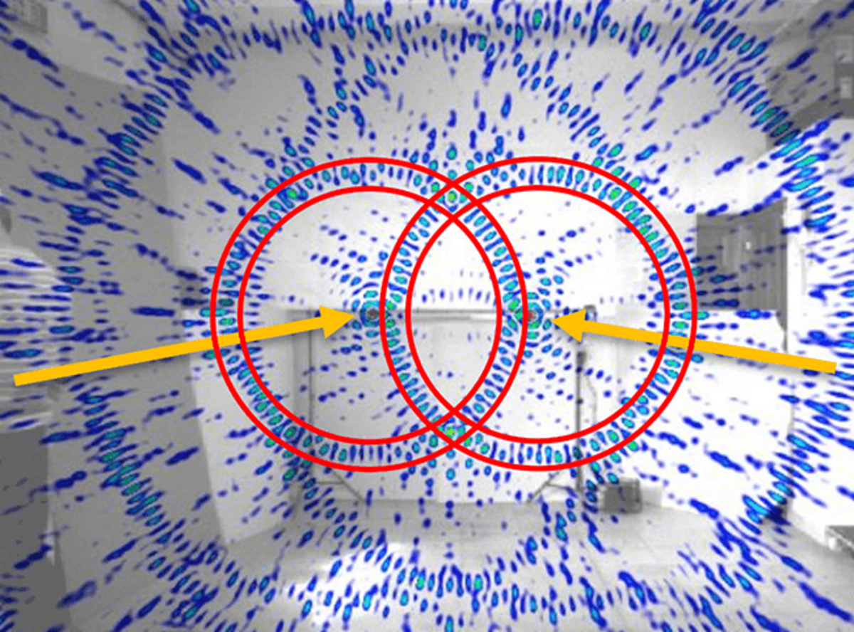
Spatial aliasing occurs primarily in arrays with equidistant microphones. To avoid this effect, the microphones should ideally all be spaced at different distances from each other e. g. using a random microphone distribution. In practice, the upper frequency limit due to local aliasing leads to limitations but still allows accurate sound source localization. Fig. 3 shows the localization of two ultrasonic sources (44 kHz) with a microphone array Ring48 (diameter 0.75 m). Even if obvious aliasing effects can be seen (e.g. within the red circles), the sources (yellow) can still be localized.