The aim of noise reduction is to reduce the effects of external noise occurring in beamforming results and thus to improve the quality (dynamic range) of the acoustic maps. For this purpose, there are evaluation methods in the time domain as well as in the frequency domain. In the following, a method applied in the frequency domain is presented.
If beamforming is performed in the frequency domain with the cross-spectral matrix (CSM), it is possible to isolate the noise computationally. The corresponding approach is based on the assumption that the noise between the different microphones of the array is uncorrelated. In this case, the noise is only found in the auto power spectra of the microphones and thus on the main diagonal of the CSM. Under the influence of various causes of noise, the auto power spectra can be much larger in magnitude than the cross power spectra and thus mask the actual source information.
Thus, to minimize the influence of noise, the diagonal elements of the cross-spectral matrix can get set to zero, which often leads to a significant improvement of the signal-to-noise ratio and reduces "ghost sound sources". A major disadvantage of this method is that by removing the main diagonal, the acoustic map is also distorted in terms of its sound level or sound power.
Application Example: Wind-Tunnel Measurements
The following example shows a wind tunnel measurement at 140 km/h wind speed. The measurement data was made available with the kind support of China Automotive Engineering Research Institute Co., Ltd. The results were calculated using standard beamforming in the frequency domain with and without the diagonal of the CSM. The frequency range goes from 1.775 kHz to 11.221 kHz.
Comparing figures 1 and 2 illustrates that, with the same dynamic range (15 dB), the signal-to-noise ratio is significantly increased when calculated without diagonal. This improves the localization of the sound sources and increases the dynamic range of the acoustic map.
Fig. 3 shows the disadvantage of this method. If the spatially averaged spectra of the first two figures are formed and compared with each other, the power loss and thus the level change are clearly visible. This influence can also be found in the maximum levels of figures 1 and 2.
 China Automotive Engineering Research Institute Co., Ltd.")
 China Automotive Engineering Research Institute Co., Ltd.")