Integration Time

The quality of a resulting acoustic map of the NoiseImage PassBy 2D module depends primarily on the integration time. It determines the length of the signal which is used for analysing each of the \(n\)=1...,N possible source points. Similarly, integration time can be interpreted as the length of the trajectory (scan width) on which one possible sound source \(n\) is tracked by the microphone array. A general prediction of a suitable integration time cannot be provided since it depends directly on the velocity \(v\) of the measured object.

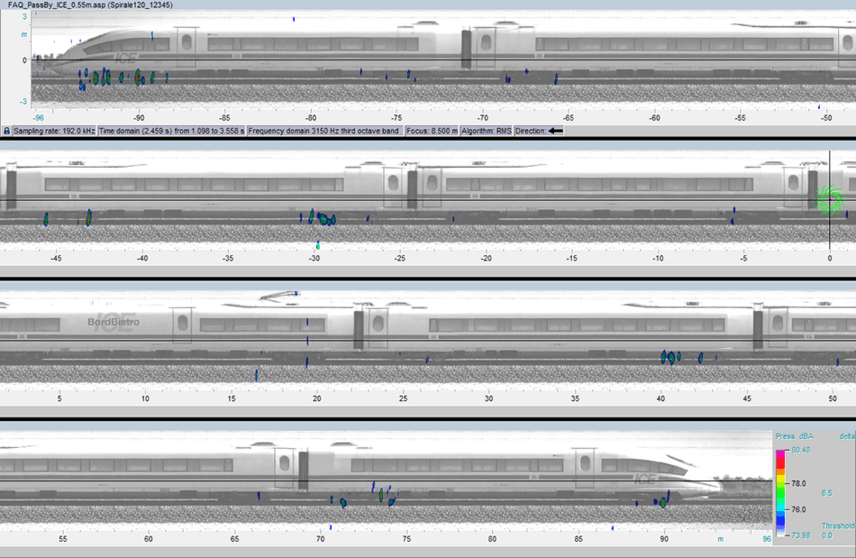
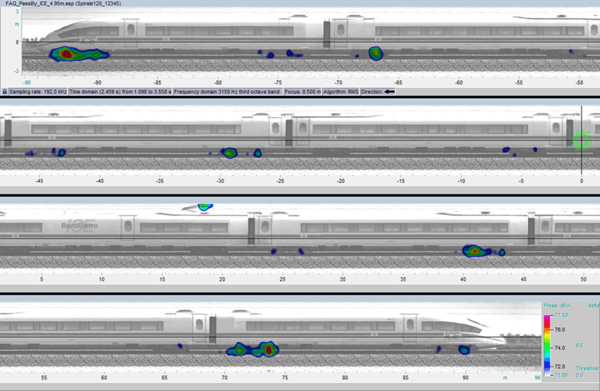
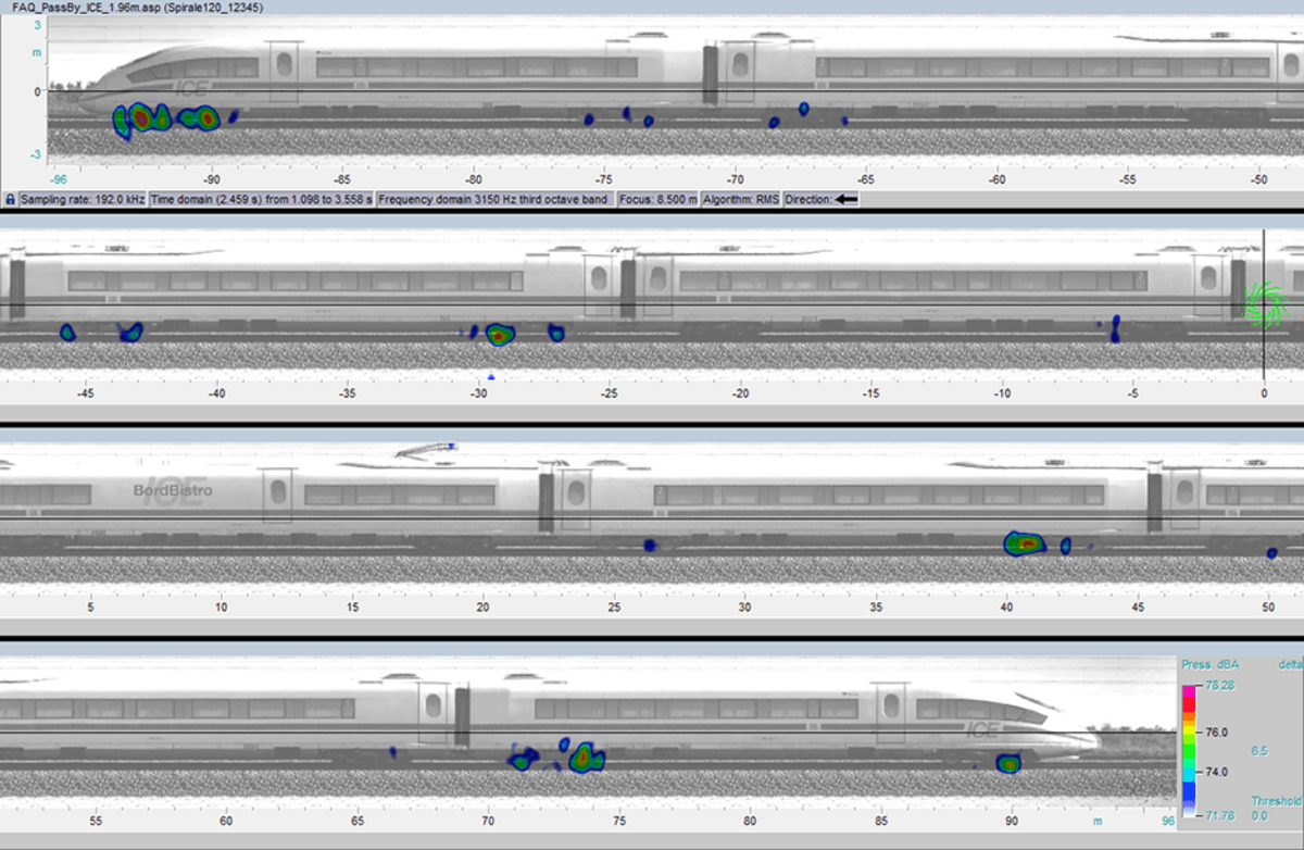
As an application example, the results of a high speed train with an average velocity of
\(v\)=78.6 m/s and different integration times are shown for the third octave band at 3.15 kHz and dynamics of 6.5 dBA. A short integration time of 7 ms (corresponds to scan width of 0.55 m, see Figure 1) may lead to a source representation which divides large connected sound sources such as the wheel set into a group of single sources. Furthermore, the number of analysed samples becomes too small to represent even a single period at low frequencies. However, long integration times such as 63 ms (corresponds to scan with of  4.95 m, see Figure 2) lead to a decrease of the acoustic maps dynamics and to a blurry source representation. Additionally, calculation time increases with a long integration time. A solution with reasonable source representation and calculation time can be found at an integration time of 25 ms (corresponds to scan width of 1.96 m, see Figure 3).