Correlation Analysis

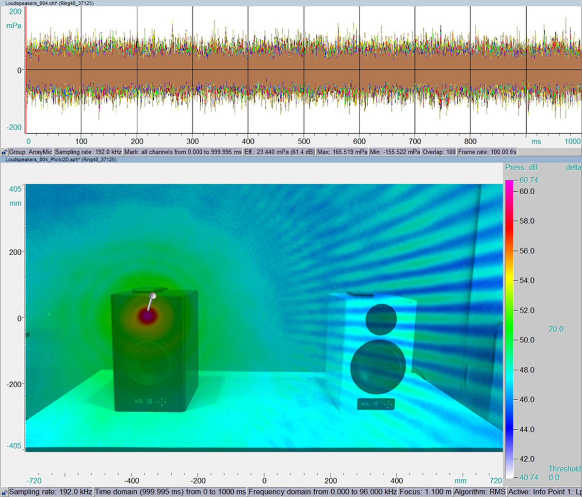
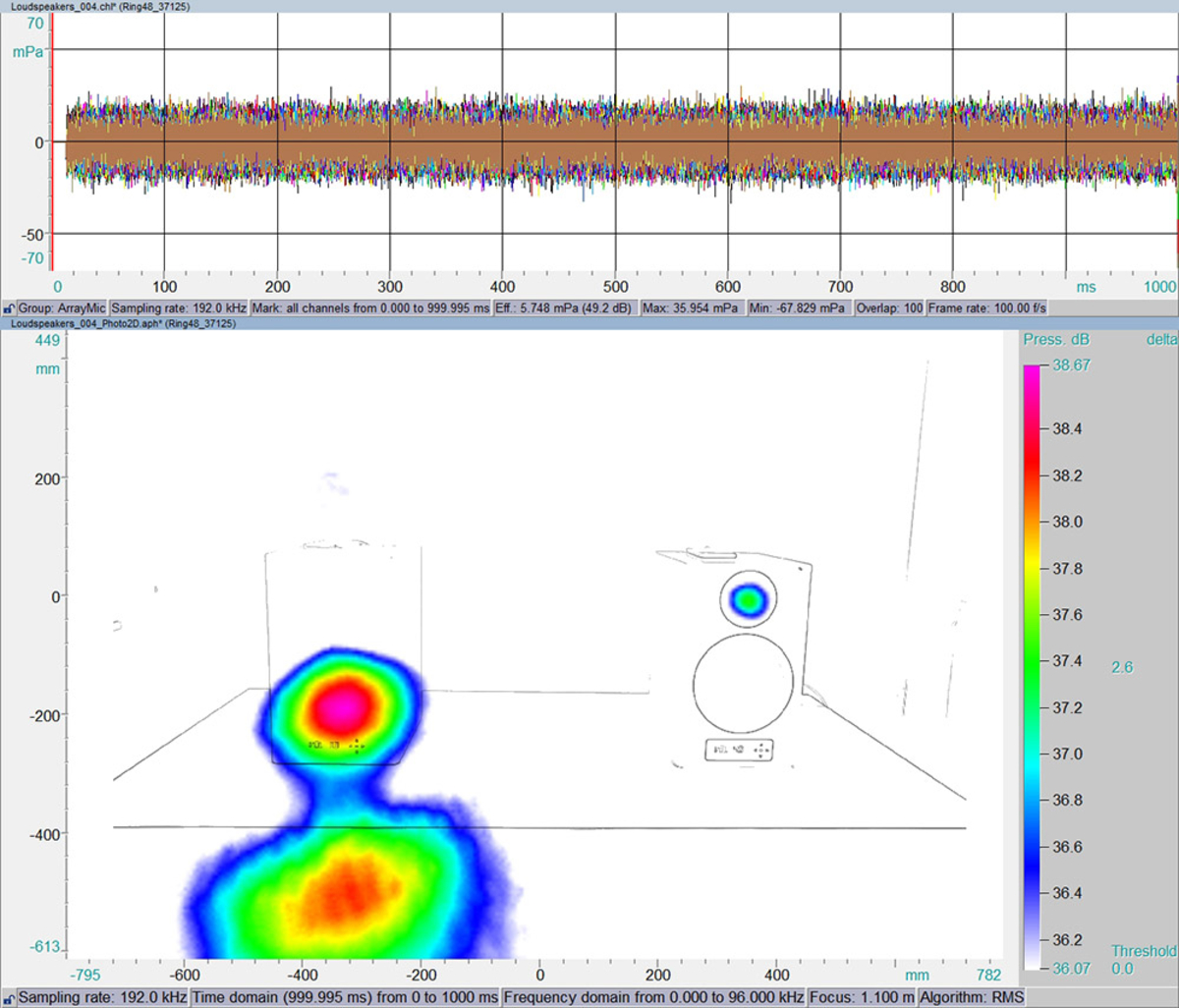
Acoustic cameras are being widely used to localize sound sources originating from any object. The sound waves picked up by the microphones can be transferred to digital signals in order to be post processed with beamforming algorithms. Those algorithms use different methods to localize the captured sound. The location of the sources will then be represented in a so-called acoustic photo which illustrates the amplitude of each source with a color scale [Figure 1].

Cross-correlation is a measure of similarities between two signals and describes the mutual relationship between two signals. On the other hand, auto-correlation is a measure of similarities of a signal with itself containing a time lag. In order to perform cross-correlation with the data of a microphone array, a reference signal is needed which can e.g. be an external microphone or an accelerometer. Therefore, the correlation function will be calculated between the signals from the microphone array and the reference signal one by one.

Figure 1 depicts the time-signals of 48 microphones captured by the microphone array Ring48 on the top and the related acoustic photo below. It shows the dominant sound source originating from a loudspeaker with a subwoofer generating white noise (20 Hz-22 kHz). The second loudspeaker with a subwoofer on the right side of the picture is 23 dB quieter than the main source, therefore it is masked by the sidelobes of the first loudspeaker.

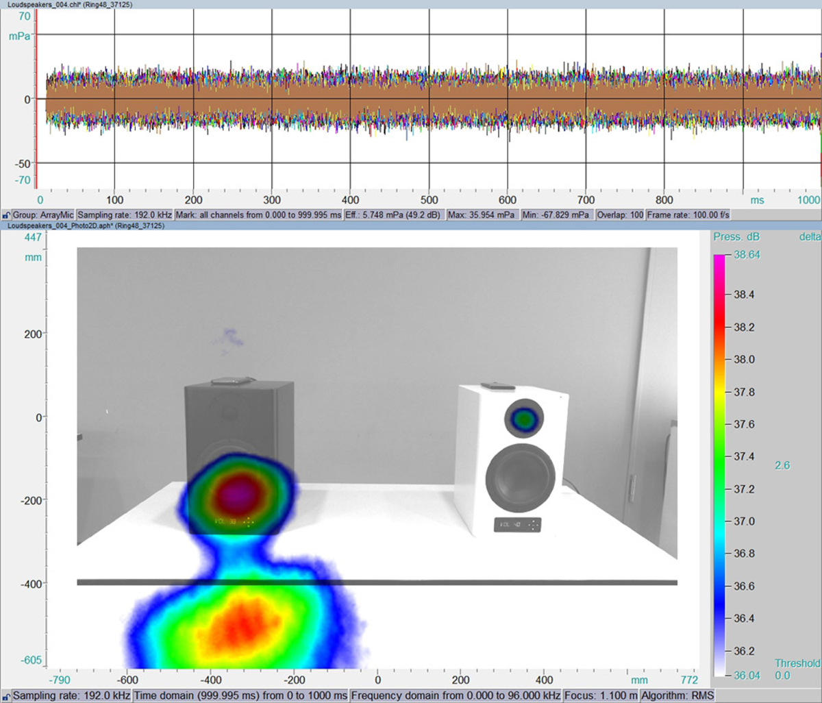
For the purpose of investigating other sound sources originating from the subwoofer and the second loud speaker, correlation analysis can be performed with the software NoiseImage.

In the software NoiseImage there are three ways to add a reference channel to perform correlation analysis with the microphone array data:

1. From an additionally recorded channel of e.g. a microphone or accelerometer
2. From a file
3. From a virtually generated reference channel directly in the acoustic image

This article will discuss the 3rd option.

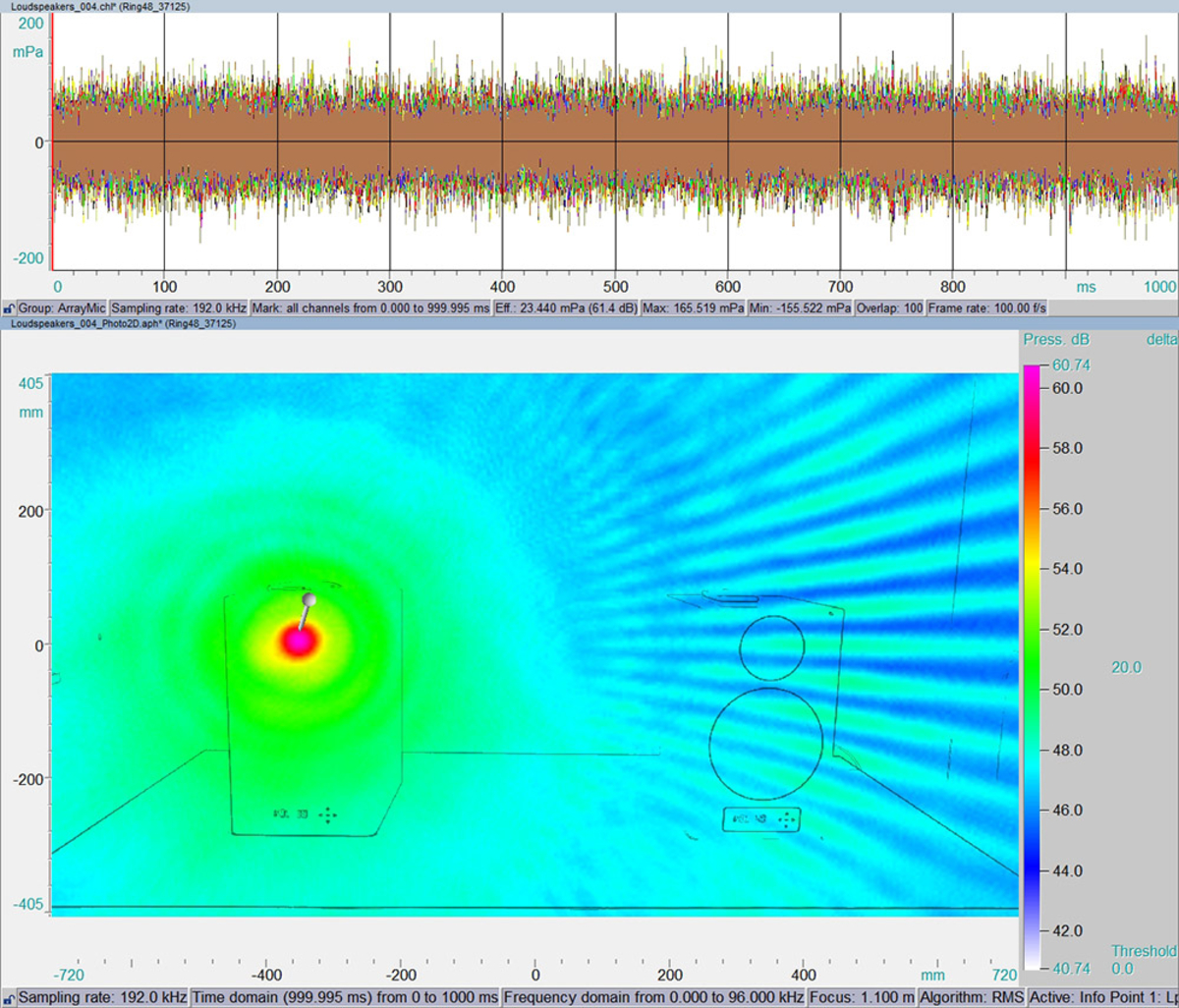
The software NoiseImage makes it possible to define a virtual reference channel on an arbitrary point in the acoustic photo and extract the beamformed signal from that point. As you can see, the reference channel was placed on the location of the dominant source in figure 1 and the corresponding signal was used as the reference signal for the correlation analysis.

After calculating the correlation function, the similarities (correlating components) between the reference channel and microphone signals can either be emphasized or deleted. Figure 2 shows the acoustic photo after deleting the correlating parts between the microphone array signals and the virtual reference channel. As expected, there is a high percentage of correlation between the dominant source and the virtual reference at the exact position of this source. So, with deleting these components from the microphone array signals the source from the first loudspeaker is vanished. The result shows three other sources: the source from the subwoofer, the reflection from the subwoofer on the table and the 23 dB quieter source from the second loudspeaker. As you can see the emission of the subwoofer is not correlated to the main tweeter source as they differ in the frequency band.

It has been shown that correlation analysis is a straightforward approach to find masked sources and increase the dynamic range of the acoustic photo. A ring configuration delivers a dynamic range between 7-10 dB but with this method we easily achieved a dynamic range of 24 dB. In many industrial applications, finding masked sources is of high interest and the user can benefit with this approach.